Making Dr GRPO go brrr

02 Jun, 2026

I wrote a fused decode-attention kernel for an RL training loop, got it 2.2× faster than the SDPA path it replaces at the microbenchmark level, dropped it into HuggingFace's generate, and watched the decode step get nearly 3× slower. The kernel was doing exactly what the microbench said it would. The integration broke an auto-compile path that the baseline was quietly benefiting from. This post is how I got there, what the gap actually was, and what closing it would have cost.

The wider context: this is the writeup of a project to RL-train a small open source model on GSM8K and write CuteDSL kernels for whichever paths dominate. The concrete setup is Qwen2.5-0.5B-Instruct, Dr. GRPO, a single A10G. The post covers two things: building the training loop from scratch (and squeezing 4.8× out of the rollout phase before any kernel work), and then writing the kernel above for the path that still dominated. Most of what follows is what those two facts look like sitting next to each other.

What is RL post-training, and why is it slow

In RL post-training for LLMs, you have a policy (the model), a verifier (something that scores outputs), and a loop that pushes the policy to produce higher-scoring outputs. For a math task like GSM8K, the verifier is just a regex that pulls the final number out of the model's response and compares it to the ground truth.

Each training step has two phases.

Rollout. Sample a prompt. Generate G completions from the current policy. Score them. Compute advantages.

Update. For K inner epochs: forward pass through the policy, compute the GRPO loss against the rewards, backprop, optimizer step.

Rollout dominates wall time. The reason is structural. Update is one big batched forward pass over (B*G, P+C) tokens, then a backward and a step. That's three GPU calls. Rollout is model.generate, which is a sequential decode loop that runs one forward pass per generated token, with each pass operating on (B*G, 1, hidden) plus a growing KV cache. Per-token compute is small, but you do it max_new_tokens times in serial. Even with KV cache and batching, you can't parallelize across the time dimension because each token depends on the last.

So most of the time, the GPU is doing many small forwards instead of a few big ones. That's the shape of the problem and that's what kernel work has to address.

PPO

PPO is a policy gradient method. You collect a rollout from the current policy, then run K epochs of mini-batch updates on that same rollout. Vanilla policy gradient is on-policy: collect a batch, do one update, throw the data away. PPO lets you reuse the same rollout for K epochs, which is the whole reason it exists, by clipping the importance ratio so the policy can't drift too far from the one that generated the data.

The ratio is

$r_{t} (θ) = \frac{π_{θ} (a_{t} | s_{t})}{π_{θ_{old}} (a_{t} | s_{t})}$

If $r_{t} = 1$ nothing changed. If $r_{t} > 1$ the new policy made the action more likely. The clipped objective is

$L^{CLIP} (θ) = {\hat{𝔼}}_{t} [min (r_{t} {\hat{A}}_{t}, clip (r_{t}, 1 - ϵ, 1 + ϵ) {\hat{A}}_{t})]$

The min picks the more conservative of the two surrogates, so PPO can improve, but not too much in one step.

Classical PPO also has a value network that estimates $V (s_{t})$ , with the advantage computed as ${\hat{A}}_{t} = R_{t} - V_{ϕ} (s_{t})$ (often via GAE).

GRPO

GRPO drops the value network. Instead of asking "is this output good?" it asks "is this output better than the others I sampled for the same prompt?".

The pipeline:

Sample $G$ completions for the same prompt
Score them with a verifier
Compute the advantage as $A_{i} = (R_{i} - μ) / σ$ inside the group
Apply the same PPO clipped objective
No critic at all

The whole machinery of estimating $V$ and computing GAE goes away because the group itself acts as the baseline.

Dr. GRPO

GRPO has two bias problems.

Length bias. The original loss averages per-response by $\frac{1}{| o_{i} |}$ . When $A_{i} < 0$ , longer responses get a weaker per-token penalty. The model learns "if I'm going to be wrong, be wrong at length." Output length drifts upward over training even when quality does not improve.

Difficulty bias. Dividing by $σ$ inside a group amplifies gradients on prompts with small std (very easy or very hard ones). Medium-difficulty groups, where the most useful learning signal lives, get under-weighted.

Dr. GRPO removes both denominators:

$A_{i} = R_{i} - μ$

and uses token-sum aggregation instead of per-response mean. The clipped objective stays the same.

L_{Dr.GRPO} (θ) = \frac{1}{G} \sum_{i = 1}^{G} \sum_{t = 1}^{| o_{i} |} min (r_{i, t} A_{i}, clip (r_{i, t}, 1 - ϵ, 1 + ϵ) A_{i})

Two deletions, no other changes.

In pseudo-code, the whole thing looks like this:

for step in range(num_steps):
    # rollout
    prompts = sample(dataset, batch_size)
    completions = policy.generate(prompts, num_samples=G)
    rewards = verifier(completions)
    advantages = rewards - group_mean(rewards)         # no std division

    old_logprobs = policy.logprobs(completions).detach()
    ref_logprobs = ref_policy.logprobs(completions).detach()

    # update
    for _ in range(K):
        logprobs = policy.logprobs(completions)
        ratio   = exp(logprobs - old_logprobs)
        surrogate = min(ratio * advantages,
                        clip(ratio, 1-eps, 1+eps) * advantages)

        loss = -token_sum(surrogate * completion_mask).mean()   # not token_mean
        loss += beta * kl(logprobs, ref_logprobs)

        optimizer.step(loss)

Three things to notice in this pseudo-code, because each one is where Dr. GRPO and most working implementations differ from the textbook description:

The advantage is rewards - group_mean(rewards). No std normalization.
The aggregation is token_sum, not token_mean. Dr. GRPO uses sum (or sum divided by a constant L_max); original GRPO uses sum divided by |o_i|.
A KL penalty against a frozen reference policy is added on top. Dr. GRPO drops this for the R1-Zero setup, but for an instruct-tuned starting point you almost always want it. I keep it.

Implementation in PyTorch

I'm using Qwen2.5-0.5B-Instruct as the policy, GSM8K as the task, and a single A10G as the hardware. The whole script (grpo.py) is around 300 lines.

I built the loop as a skeleton first. No real rewards, no real loss math, just the shape. The point was to get something running end to end with torch.rand rewards and fake advantages, so I could replace each function with the real one once the surrounding scaffolding worked.

The skeleton:

Load the model and the dataset
Sample completions
Compute fake rewards
Compute fake advantages
Compute loss
loss.backward()
optimizer.step()

Once this ran without errors, I replaced each function with the real one. Three of those replacements had non-obvious gotchas worth writing down.

The completion mask

generate pads with EOS after the model finishes. I needed a mask that's 1 for real tokens and 0 after the first EOS, so the loss does not credit the model for padding.

From grpo.py:

def build_completion_mask(completion_ids, eos_token_id):
    is_eos = completion_ids == eos_token_id
    has_eos = is_eos.any(dim=1)
    first_eos_idx = is_eos.float().argmax(dim=1)
    seq_len = completion_ids.shape[1]
    positions = torch.arange(seq_len, device=completion_ids.device).unsqueeze(0)
    mask = (positions <= first_eos_idx.unsqueeze(1)).long()
    mask = torch.where(has_eos.unsqueeze(1), mask, torch.ones_like(mask))
    return mask

The torch.where at the end is the gotcha. argmax returns 0 when there's no True in the row, so without the fallback, completions that never emit EOS would get a mask of [1, 0, 0, ...] and only the first token would count. The where says: if the row has no EOS at all, treat the whole completion as real.

compute_logprobs

To compute $\log π_{θ}$ for the sampled tokens, I concatenate prompt and completion, run a forward pass, and gather the log-probs at the right positions.

The off-by-one trap: logits at position $t$ predict the token at $t + 1$ . So the logits that score the completion are at positions $[P - 1, P, . . ., P + C - 2]$ , not $[P, P + 1, . . .]$ .

From grpo.py:

def compute_logprobs(model, prompt_ids, prompt_attention_mask, completion_ids, completion_mask):
    B, P = prompt_ids.shape
    BG, C = completion_ids.shape
    G = BG // B
    device = completion_ids.device

    prompt_ids_expanded = prompt_ids.repeat_interleave(G, dim=0).to(device)
    prompt_attn_expanded = prompt_attention_mask.repeat_interleave(G, dim=0).to(device)

    full_ids = torch.cat([prompt_ids_expanded, completion_ids], dim=1)
    attention_mask = torch.cat([prompt_attn_expanded, completion_mask], dim=1)

    logits = model(input_ids=full_ids, attention_mask=attention_mask).logits
    completion_logits = logits[:, P - 1 : P - 1 + C, :]

    log_probs = F.log_softmax(completion_logits, dim=-1)
    selected = log_probs.gather(dim=-1, index=completion_ids.unsqueeze(-1)).squeeze(-1)
    return selected

I verified this by feeding prompt + completion[:5] through the model manually, taking the last logit row, and comparing to selected[0, 5]. They matched to bf16 precision (~4e-3 difference). That sanity check was worth the ten lines it took to write, because every other piece downstream depends on these log-probs being right.

The loss

Once compute_logprobs worked, the loss was a direct translation of the equation.

From grpo.py:

def grpo_loss(current_logprobs, old_logprobs, advantages, completion_mask, eps=0.2):
    ratio = torch.exp(current_logprobs - old_logprobs)
    advantages = advantages.unsqueeze(1)
    unclipped = ratio * advantages
    clipped = torch.clamp(ratio, 1 - eps, 1 + eps) * advantages
    per_token_loss = -torch.min(unclipped, clipped)
    masked_loss = per_token_loss * completion_mask
    loss_per_response = masked_loss.sum(dim=1)
    return loss_per_response.mean()

Two details that are easy to get wrong:

The mask multiplies per_token_loss, not ratio. Masking the ratio destroys exp(0) = 1 at padded positions, which silently changes the surrogate at every step rather than just zeroing out padding contributions.

Clip the ratio, then multiply by advantage. Clipping ratio * advantage is a different operation and does not give you PPO.

On inner step 0, current_logprobs equals old_logprobs, so ratio is exactly 1 everywhere and the loss reduces to -(advantages * mask).sum(dim=1).mean(). I print this every run as a sanity check that nothing in the graph is detached or wrong.

Putting it together

With those three helpers, the full naive GRPO step is short.

From grpo.py:

for step in range(EPOCHS):
    questions, gold_answers = sample_batch(dataset, BATCH_SIZE)
    prompts = [format_prompt(q, tokenizer) for q in questions]
    tokenized = tokenize(prompts, tokenizer)

    completion_ids = generate_completions(
        model, tokenized["input_ids"], tokenized["attention_mask"], tokenizer
    )
    mask = build_completion_mask(completion_ids, tokenizer.eos_token_id)

    rewards, decoded = compute_rewards(completion_ids, gold_answers, tokenizer, G)
    B = len(questions)
    rewards_grouped = rewards.view(B, G)
    advantages = (rewards_grouped - rewards_grouped.mean(dim=1, keepdim=True)).view(B * G)

    with torch.no_grad():
        old_logprobs = compute_logprobs(model, ..., completion_ids, mask)
        ref_logprobs = compute_logprobs(ref_model, ..., completion_ids, mask)

    for inner in range(K):
        current_logprobs = compute_logprobs(model, ..., completion_ids, mask)
        kl = masked_kl(current_logprobs, ref_logprobs, mask)
        loss = grpo_loss(current_logprobs, old_logprobs, advantages, mask) + BETA * kl

        optimizer.zero_grad()
        loss.backward()
        torch.nn.utils.clip_grad_norm_(model.parameters(), max_norm=1.0)
        optimizer.step()

A few notes on what's there:

old_logprobs is computed once per outer step under torch.no_grad() and reused across the K inner updates. This is the same rollout policy that produced the completions. Freezing its log-probs is what gives the PPO ratio meaning.

ref_logprobs is computed against a frozen copy of the initial model. The KL term BETA * masked_kl(current, ref, mask) is what keeps an instruct-tuned policy from drifting too far from its starting point, which is what most papers do for non-R1-Zero setups. I use the k3 estimator from Schulman: kl = exp(ref - current) - (ref - current) - 1, which is non-negative and unbiased.

The advantage computation is the only place where the implementation diverges from original GRPO. Original GRPO would have one extra line:

advantages = (rewards_grouped - rewards_grouped.mean(dim=1, keepdim=True)) / (rewards_grouped.std(dim=1, keepdim=True) + 1e-8)

and the loss aggregation would be masked_loss.sum(dim=1) / mask.sum(dim=1). Both are removed in Dr. GRPO. That's the whole simplification.

Real rewards

For GSM8K the gold answer is whatever number appears after #### in the answer field. I parse both the gold answer and the model output with the same regex and assign:

1.0 for correct answer in the right format
0.1 for correct format, wrong number
0.0 otherwise

The 0.1 partial reward exists because the model is unlikely to get math right early in training. Without it, every group has all-zero rewards, every advantage is zero, every loss is zero, nothing learns. The format reward gives the model something to climb before the math reward kicks in.

The cold start

The first 1000-step run with Qwen showed eval_exact_match at 0.0 across all 40 evaluations. Format rate hovered near zero. With the chat template applied via apply_chat_template and an instruct-tuned model, this should have been a solved problem. It wasn't.

(Aside: I had spent a few days before this trying to get SmolLM2-135M to do GSM8K. It can't, and that's a clean a priori finding rather than a Dr. GRPO finding. A 135M base model has neither the math nor the instruction-following to start RL from. The switch to Qwen2.5-0.5B-Instruct was supposed to fix the instruction-following half. It did not, for the reason below.)

The reason was visible in a single sample completion. Qwen2.5-Instruct is math-tuned and wants to write in LaTeX:

Emily's total score for this assignment:
\[ 9 \times 92 = 828 \]

It also wants to use \boxed{} rather than ####. The system prompt's request for #### NUMBER was too soft to override the math-tuning prior, and the regex was too narrow to catch what the model actually emitted. I broadened the regex to match ####, \boxed{...}, answer is N, and = N, with findall plus last-match so intermediate calculations don't beat the final answer.

From grpo.py:

ANSWER_RE = re.compile(
    r"(?:####|\\boxed\{|answer is\s*:?\s*|=)\s*\$?(-?\d+(?:\.\d+)?)\$?\}?",
    re.IGNORECASE,
)

def extract_answer(text):
    matches = ANSWER_RE.findall(text)
    return matches[-1].strip() if matches else None

I also strengthened the system prompt with the format requirement at the end of the instruction (recency bias) and explicit prohibitions of LaTeX and \boxed.

This got format rate up. Exact match did not move. The 0.5B model is just not strong enough at math for GSM8K to be a useful signal at this scale.

Results

Before going further, a note on scope. The 0.5B model is too small to actually learn GSM8K within reasonable training budgets, and I'm not pretending otherwise. What this post is about is the loop's performance, not its accuracy. The training run below exists to validate that the implementation is correct; the speedup work later is the actual contribution.

wandb dashboard part 1

wandb dashboard part 2

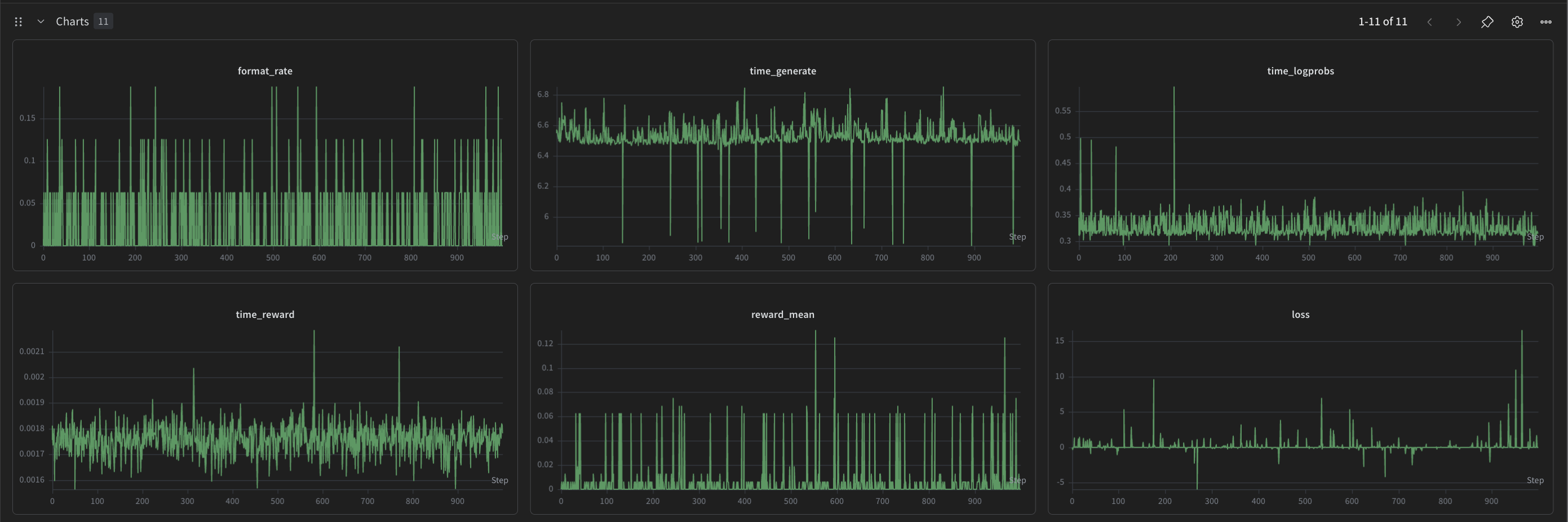
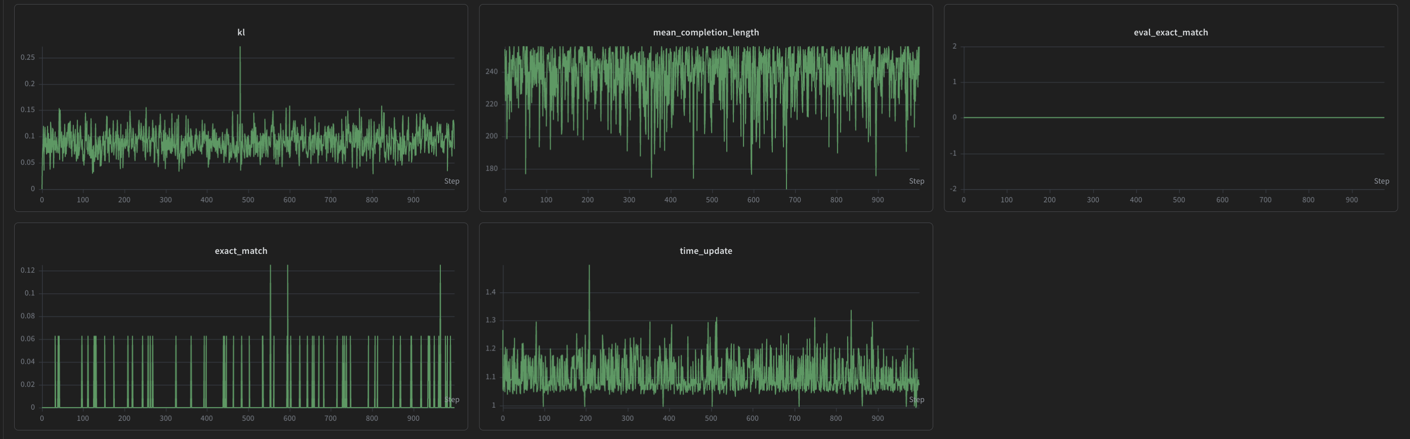
What's in these charts:

eval_exact_match stays near 0 the whole run. The 0.5B model cannot reliably solve GSM8K problems.
format_rate is high from step 0 because the broadened regex catches LaTeX/boxed answers, not because RL is teaching anything.
mean_completion_length stays stable rather than drifting upward.
kl against the frozen reference grows slowly, as expected, indicating the policy is genuinely moving but the KL regularizer is keeping the drift reasonable.
loss is well-behaved (no spikes). Grad clipping at 1.0 is doing its job.

The mean_completion_length stability is worth pausing on. Under vanilla GRPO this would drift upward over training. That's the length bias Dr. GRPO is designed to remove. The fact that it doesn't drift here, on a model too small to actually improve at the task, is about as clean a demonstration of the bias-1 fix as you can get: the only signal in the data is the algorithmic effect, with no confound from the model actually learning. I didn't set this up as an experiment. It fell out of running the wrong-sized model.

The implementation passes every sanity check I've thrown at it: ratio is exactly 1 on inner step 0, manual log-prob computation matches compute_logprobs, the mask correctly handles both EOS-terminated and length-truncated completions, and the loss is exactly zero in the degenerate B=1 case where advantages sum to 0 within the group.

The point of this run isn't the learning curve. It's that the loop is verified correct and the timing data is real. From the per-step breakdown:

gen=~6.5s  reward=~0.00s  logprobs=~0.32s  update=~1.07s

Generate is 82% of step time. That is the headline number for the rest of the project.

Profiling

The "generate is 82% of step time" headline from the previous section came from coarse time.perf_counter() brackets. That's enough to know which phase to look at, but it doesn't tell me which kernels are running, how big they are, or where the gaps between them are. For that I need a real profiler.

I'm using PyTorch Profiler with record_function annotations around each phase. The skeleton:

from torch.profiler import profile, record_function, ProfilerActivity

with profile(
    activities=[ProfilerActivity.CPU, ProfilerActivity.CUDA],
    record_shapes=True,
    with_stack=True,
    schedule=torch.profiler.schedule(wait=1, warmup=1, active=3, repeat=1),
    on_trace_ready=torch.profiler.tensorboard_trace_handler("./profile_traces"),
) as prof:
    for step in range(5):
        with record_function("rollout"):
            # generate_completions
            ...
        with record_function("reward"):
            # compute_rewards
            ...
        with record_function("logprob_old"):
            # old_logprobs forward pass
            ...
        with record_function("logprob_ref"):
            # ref_logprobs forward pass
            ...
        with record_function("update"):
            for inner in range(K):
                with record_function(f"update_inner_{inner}"):
                    # current_logprobs + loss + backward + step
                    ...
        prof.step()

A few notes on the choices:

schedule(wait=1, warmup=1, active=3, repeat=1) skips step 0 (cuDNN / kernel-selection noise), warms up once, then profiles 3 active steps. That's enough because the per-step kernel pattern repeats.
with_stack=True and record_shapes=True give the most informative trace but blow up the file size. My 5-step trace came out to 4 GB. Worth it for the first pass.
The record_function blocks wrap each pipeline phase so the trace shows labeled spans instead of an undifferentiated wall of kernels.

Here's the resulting view:

Profiling Results

The first time I opened this I bounced off it hard. A profiler trace is dense and it isn't obvious where to start looking. I posted about it and got some useful pointers on how to read this kind of output:

Twitter Replies

The trace covers 3 active profiler steps (steps 2–4, after 1 skip + 1 warmup as configured). Each step is ~15.1s. Here is the per-step time budget, averaged across all three:

generate:     13.63s   90.3%
update:        1.17s    7.7%
logprob_old:   0.16s    1.0%
logprob_ref:   0.15s    1.0%
reward+setup:  0.00s    0.0%

Generate isn't just the slow part. It's basically the only part.

Inside generate

Each generate call runs 256 decode steps, one forward per token. The profiler caught 768 of these forwards in total (256 forwards per call × 3 profile steps), each averaging 49.5ms on the CPU side. That 49.5ms is wall-clock per forward as seen from the CPU thread. Most of it is the CPU waiting for the previous step's GPU work to complete enough to dispatch the next, not pure CPU dispatch time. At 26.6% GPU utilization the CPU↔GPU overlap is small, so per generate call that 256 × 49.5ms ≈ 12.7s figure is a fair total-time accounting.

The full-sequence forwards used by logprob_old, logprob_ref, and the update inner loop average 89.6ms each. Nearly double a single decode forward, but they only run 9 times total across the trace, vs. 768 per-token decode forwards. That's the trade: a handful of batched full-sequence forwards vs. hundreds of per-token forwards, even though each individual decode forward is "cheaper" per call.

The headline number from the trace is GPU utilization: 26.6%. Over the 45.5s kernel span, the GPU was running a kernel for 12.1s and idle for 33.4s. Median gap between consecutive kernels is 23.6µs. P90 is 72µs. The GPU is starving for work.

The dispatch counts make it concrete:

aten::linear / matmul / mm   342,108 calls
  under 50µs                  59.2%
  under 100µs                 99.1%
  over 1ms                     0.1%

The under-50µs bucket is the decode-step GEMMs: at each of the 256 token positions, 24 layers each fire a (B*G, 1, hidden) matmul. That's high launch count, low arithmetic intensity, and the GPU spends more time loading weights than doing math.

So the bottleneck has three layered causes: the decode is sequential (can't parallelize across time without speculative decoding or similar), each step is memory-bound (the GEMMs are too small to saturate compute), and the CPU can't dispatch fast enough to keep the GPU fed.

Baseline cleanup

Before writing kernels, I wanted to clear the obvious Python-side waste. Three changes, in order. Each one is a separate runnable file in the repo: vanilla, +torch.compile, +pinned tensors, +static KV cache. Each diff is small and shows exactly one change against the previous.

1. torch.compile. Wrap the policy and ref model with torch.compile(dynamic=True, fullgraph=False). First attempt used mode="reduce-overhead" (which enables CUDA graph capture). That blew up the trace to 22M events and dropped GPU utilization to 18.6%, because the dynamic KV cache shapes were breaking the graph cache and triggering 6 recompiles inside the active profile window. Dropping reduce-overhead fixed it.

                  baseline   +compile
GPU utilization   26.6%      24.7%
generate avg      13.63s     14.10s
update avg        1.17s      0.84s   (-28%)
logprob avg       89ms       25ms    (-72%)

The update phase improved nicely. Generate didn't move. HuggingFace's generate loop has enough Python control flow (sampling, stopping criteria, KV bookkeeping) that Dynamo hits graph breaks at the same points whether compile is on or off. The 768 token-step forwards look identical in the kernel trace.

This is actually more useful than a speedup would have been. torch.compile helps where the shapes are predictable and the graph is unbroken, which is exactly the update phase. The decode loop is the opposite: sequential, dynamic shapes, Python control flow.

2. Pin tensors on device. tokenize() was returning CPU tensors and every downstream function was calling .to(DEVICE) on its own. compute_logprobs did it on the repeat_interleave-expanded prompts, which means once per logprob_old, once per logprob_ref, and once per inner update step. Four extra transfers per training step, all of the same data.

Fix: move .to(DEVICE) once into rollout_setup and delete the rest. Note that .to(device) is not free even when the tensor already lives on the right device. It still goes through ATen dispatch.

                  +compile   +pinned
device transfers  13.97s     10.04s   (-28%)
stream syncs      2.55s      1.01s    (-60%)
GPU utilization   24.7%      23.6%

Transfer and sync overhead dropped exactly as expected. But rollout_setup jumped from 2ms to 125ms. Front-loading .to(DEVICE) made the transfer synchronous instead of letting it overlap with subsequent work. Generate is still 14.66s. Net effect on step time: near zero.

3. Pre-allocate the KV cache. This is the one that mattered.

The default KV cache in generate grows the K/V tensors at each decode step via aten::cat. That produces a new tensor shape every step, which is exactly what was breaking Dynamo's graph cache. Switching to StaticCache pre-allocates (batch, heads, max_seq_len, head_dim) upfront and writes K/V slices in place.

From profile_grpo_static_kv_cache.py:

past_key_values = StaticCache(
    config=model_config,
    max_batch_size=BATCH_SIZE * G,
    max_cache_len=max_prompt_len + MAX_NEW_TOKENS,
    device=DEVICE,
    dtype=torch.bfloat16,
)

With fixed shapes, the decode-step graph is traceable. Dynamo captures once and replays it for all 256 steps.

                  baseline   +compile   +pinned    +static KV
GPU utilization   26.6%      24.7%      23.6%      86.2%
generate avg      13.63s     14.10s     14.66s      2.81s
matmul dispatches 342K       339K       339K        5.4K
KV cat calls      77,994     76,830     76,830      2,481
trace size        3.9GB      3.9GB      3.9GB       765MB

Generate went from 13.63s to 2.81s. A 4.8× speedup, and GPU utilization hit 86.2%. The per-token forward dispatch dropped from 49.5ms to 1.55ms on the CPU side. The GPU is still doing roughly the same amount of work per token; the difference is that the CPU is no longer the bottleneck. Once the graph is captured, the host queues all the kernels for one decode step in microseconds and races ahead to the next one.

The new bottleneck

With the decode graph captured, a different cost surfaces:

aten::item                  4.49s   7,380 calls
aten::is_nonzero            4.48s     774 calls
aten::_local_scalar_dense   4.48s   7,380 calls

These are scalar D2H reads. At every decode step, HuggingFace's generate loop calls .item() on a boolean tensor to check whether all sequences have hit EOS. That forces a host-side wait for the GPU. With the compiled forward, this stopping-criteria check is now the dominant cost inside generate.

You can't fix this with compile or caching. It's structural to how HF implements generate. The two options are: replace model.generate with a custom decode loop that keeps the stopping check on the GPU, or take 86.2% utilization as the new floor and move to the kernel work.

For the purpose of this post, that's the cleanest baseline I'm going to get without rewriting generation from scratch. Time to write kernels.

Optimization 1: Fused decode attention with RoPE and KV-cache write

A note on naming up front, because I use three terms more or less interchangeably below: SDPA is the PyTorch API (F.scaled_dot_product_attention), fmha_cutlassF_bf16_64x64_sm80 is the specific CUDA kernel SDPA dispatches to on Qwen2.5 shapes, and FlashAttention is the algorithmic family that kernel implements (CUTLASS port). "Replacing SDPA with my kernel," "beating the flash-attention path," and "replacing fmha_cutlassF" all refer to the same thing.

The profiling section ended on this: per-token attention is ~23% of total kernel time, currently split across two kernel launches per layer per token. One launch for a Triton wrapper that does RoPE and some elementwise prep, another for the SDPA flash kernel doing the attention math. Two launches where one is sufficient is the obvious first target.

The fused kernel does three things in one launch:

RoPE-rotate Q and the new K at the current decode position.
Write the rotated K_new and V_new into the static KV cache at position p.
Compute attention between Q and the populated prefix cache[:, :, :p+1, :].

These bundle together because they all touch the same data on the same step. RoPE reads Q and K and writes them back. The KV cache write reads K and V and writes them elsewhere. Attention reads Q and the cache. As three separate kernels that's six HBM round-trips on tensors that are conceptually live at the same instant of computation. Fused, the data stays on-chip and we pay for one launch instead of three.

I'm writing it in CuteDSL, same as the previous FA2 post. Keeping the toolchain consistent across the kernel sequence so the comparison is apples-to-apples.

Reference first

Before writing any kernel code, I wrote a PyTorch reference at experiments/decode_attention_reference.py. Same three operations, but written naively in PyTorch. Its job is to be the ground truth the kernel has to match.

The reference is verified two ways:

RoPE output matches transformers.models.qwen2.modeling_qwen2.apply_rotary_pos_emb exactly.
Attention output matches F.scaled_dot_product_attention to bf16 tolerance.

A few Qwen-specific details drop out of writing this:

head_dim = 64, num_q_heads = 14, num_kv_heads = 2. Qwen2.5 uses GQA with a 7:1 group ratio.
rope_theta = 1_000_000, not the default 10000. Hardcoding the default would have produced rotations that almost match but fail allclose.
RoPE uses the half-split rotation (rotate [d/2, d] against [0, d/2]), not adjacent pairs. The HF Qwen2 source is the canonical reference for the exact pairing.

Dtype choices

bf16 in, bf16 out, fp32 accumulators inside. Concretely:

Cosine and sine for RoPE: fp32. Trig in bf16 loses too much precision at small angles.
QK^T accumulator: fp32.
Softmax (max-subtract, exp, sum): fp32.
PV accumulator: fp32.
Final cast back to bf16 only at the store.

This is what fmha_cutlassF already does internally, and what cuBLAS does for tensor-core matmuls. The reference reproduces it with .float() upcasts before each matmul and a .to(DTYPE) at the end. Matching the reference at atol=1e-2 catches real numerics bugs before they show up in training.

The kernel

The fused kernel is short. One CTA per (batch, q_head), 32 threads per CTA (one warp), each thread owning two of the 64 head-dim slots (d0 = tid, d1 = tid + 32). Q gets RoPE-rotated into registers and stays there. The rotated K_new and V_new get written to the cache at slot position before the attention loop starts. The inner loop walks [0, position] doing online softmax against the cache.

A few choices fall out of the shapes:

32 threads is one warp. The Q·K partial sum reduces across the warp with shuffle_sync_bfly instead of going through shared memory.
One CTA per (B*G, H_Q) = (2*8, 14) = 16 × 14 = 224 blocks. The "batch" here is BATCH_SIZE × num_generations = 2 × 8 = 16 sequences, each with 14 attention heads. Small grid, but enough to keep an A10G's SMs occupied for this workload.
GQA is 7:1. Seven sibling CTAs share the same K_new and V_new. They all write the rotated K_new to the same cache slot unconditionally. Same value, same address, same warp. The race is benign because every CTA writes the same bits to the same bytes, so the final state is deterministic regardless of who "wins." The seemingly more conservative version, gating on h_q % GROUP_SIZE == 0 so only one CTA writes, is actually more racy, because the non-writing CTAs have no inter-CTA barrier against the writer and may read slot position before it's been written. The unconditional write is safe because each CTA reads back its own write inside the same thread, which is sequentially consistent in global memory and needs no fence.

It took me longer than I want to admit to convince myself of that. The instinct is "obviously you don't want multiple CTAs writing the same memory" and the answer is "yes you do, and gating it is the actually-broken version." I left the reasoning in a comment block in the kernel because future-me would rederive it otherwise.

The inner loop is the part worth showing.

From kernels/attention_with_kv_cache.py:

# online softmax state. wrap in cute.Float32 so the loop body doesn't
# silently promote to Float64 mid-iteration
m = cute.Float32(-1.0e30)
l = cute.Float32(0.0)
acc = [cute.Float32(0.0), cute.Float32(0.0)]

for n in range(position + 1):
    # partial Q·K[n], each thread contributes 2 of the 64 head-dim slots
    partial_score = (
        q_vec[0] * k_cache[b, h_kv, n, d0].to(cute.Float32)
        + q_vec[1] * k_cache[b, h_kv, n, d1].to(cute.Float32)
    )

    # warp reduce: butterfly shuffle so every lane ends up with the full sum
    score = partial_score
    for mask_off in [16, 8, 4, 2, 1]:
        score = score + cute.arch.shuffle_sync_bfly(score, mask_off, 0xffffffff)
    score = score * SCALE

    # online softmax update. keep m, l, acc in fp32
    m_new   = cute.Float32(max(m, score))
    alpha   = cute.Float32(cute.math.exp(m - m_new))
    prob    = cute.Float32(cute.math.exp(score - m_new))

    acc[0] = acc[0] * alpha + prob * v_cache[b, h_kv, n, d0].to(cute.Float32)
    acc[1] = acc[1] * alpha + prob * v_cache[b, h_kv, n, d1].to(cute.Float32)

    l = l * alpha + prob
    m = m_new

This is the standard online-softmax pattern (FlashAttention's m, l, acc variables) with the partial Q·K reduction sharded across the warp. The cute.Float32(...) wrappers around m_new, alpha, prob are not cosmetic. Without them the loop body silently promotes to Float64 after the first cute.math.exp call, which both slows the loop down and changes the numerics.

I learned that one by reading a profiler trace where the kernel was 2× slower than expected for no apparent reason.

The structure that makes this a single-warp kernel is the inner loop walking n sequentially. A multi-warp version would tile the K dimension: multiple warps each handle a chunk of [0, position], run their own local online softmax, and then merge the partial (m, l, acc) states with a single reduction at the end. That's the natural next kernel for long contexts (see the position=1023 number below), but it's a different kernel and a bigger project than I scoped here.

Full code is at kernels/attention_with_kv_cache.py.

Microbenchmarks

Compiled once via cute.compile, benchmarked against two PyTorch references at the same shapes:

Manual reference. RoPE on Q/K_new, cache write, GQA expand via repeat_interleave, then attention as matmul + softmax + matmul in fp32.
SDPA reference. Same RoPE and cache write, same GQA expand, but the attention math goes through F.scaled_dot_product_attention, which dispatches to flash-attention on these shapes. This is the path the unmodified HF Qwen2 model takes.

The kernel iterates [0, position]. The references slice [0, position+1]. All three scale with position. The interesting question is how each one scales.

Position sweep (microseconds per decode step)
   pos   ref (manual)   ref (SDPA)    kernel   ker/ref   ker/SDPA
    32          412.9        295.6     135.1      0.33       0.46
    64          415.5        295.1     134.5      0.32       0.46
   128          412.7        292.6     134.6      0.33       0.46
   256          426.5        313.5     134.5      0.32       0.43
   511          453.0        298.2     134.8      0.30       0.45
  1023          826.2        366.7     434.4      0.53       1.18

The kernel beats SDPA by a factor of ~2.2× across positions 32–511. The GRPO config caps total sequence length at MAX_PROMPT_LEN + MAX_NEW_TOKENS = 200 + 256 = 456, so position 511 is at the right edge of the "in scope" range. Within that range the kernel is a clean 2.2× win against the realistic baseline.

It loses at 1023. The single-threaded inner attention loop scales linearly. SDPA's flash kernel scales sub-linearly because it's tiled and multi-warp. For long contexts the kernel would need a tiled inner loop and a proper multi-warp reduction. That's the natural follow-up, but it's a different kernel.

Plugging it in

Replacing Qwen2Attention.forward is at experiments/qwen2_fused_attention_patch.py. When seq_len == 1 and cache_position is available, the patched forward routes the layer through the fused kernel. Anything else (prefill, training, output_attentions=True, etc.) falls back to the original implementation.

Validating the patched HF path against a direct call to the same kernel:

max abs diff:   0.0000e+00
k_cache slot:   0.0
v_cache slot:   0.0
PASS: kernel matches HF within atol=1e-2, rtol=1e-2.

Bit-exact, because both paths dispatch to the same compiled kernel under the hood. The integration is correct.

End-to-end

Patched generate, three active profiler steps, averaged:

                  baseline (SDPA)   +fused kernel
generate avg      2.81s             8.21s
GPU utilization   86.2%             37.6%

Generate got nearly 3× slower with a kernel that's 2.2× faster than SDPA at the microbenchmark level. That number is what the rest of this section is about.

Where the time goes

The profile breakdown from the patched run:

fused decode kernel       18,360 calls   1.86s   101us avg   (the kernel itself)
cudaLaunchKernel         129,042 calls   2.43s    19us avg   (per-launch CPU dispatch)
aten::is_nonzero             786 calls   1.40s  1.78ms avg   (HF stopping check, sync wait, not op cost)
aten::item                 5,805 calls   1.43s   246us avg   (scalar D2H reads, sync wait, not op cost)

The kernel runs in the expected time: 18,360 calls × 101µs ≈ 1.86s. That matches the microbenchmark almost exactly. The kernel is doing what the bench said it would.

The cost is everywhere around the kernel:

2.43s in cudaLaunchKernel. Each launch costs ~19µs of CPU dispatch. With 129k launches in a generate, that's 2.43s of CPU time just queuing work.
1.40s in is_nonzero. HF generate's stopping check calls is_nonzero on a boolean tensor every decode step. Each call averages 1.78ms in our profile, way more than the operation itself. The cost is the synchronization: the CPU has to wait for the GPU queue to drain before reading the boolean. A long queue of small launches means each sync takes longer.
1.43s in item. A mix of HF's internal scalar reads (sampling, KV bookkeeping) and the one .item() in the patched forward used to extract position for the kernel. Same root cause as is_nonzero.

The baseline (SDPA) has the same is_nonzero checks and the same sampling-side item calls. It runs in 2.81s at 86% utilization because the GPU queue is shorter; each sync drains faster when there are fewer launches queued in front of it. The difference between the two paths is what HF generate is doing around attention.

The version of HF I'm using auto-compiles the decode-step forward when a StaticCache is supplied: Dynamo + Inductor → CUDA graph capture for the shape-stable parts. In the baseline trace this shows up as ~39k cudaGraphLaunch calls alongside ~129k regular cudaLaunchKernel calls. The graph captures the embedding + norms + projections + SDPA + residual + MLP and replays them as one launch per graph fragment.

@torch._dynamo.disable on patched_qwen2_attention_forward makes the entire attention layer a graph break. Dynamo captures the embedding and the residual/MLP around attention, but the attention itself runs eager, every layer, every token. That's where the extra ~80k cudaLaunchKernel events come from. The kernel itself is a single launch, but the q/k/v/o projections and the reshapes around it become individual launches instead of one captured fragment.

Removing the disable doesn't help. Dynamo immediately graph-breaks on the .item() needed to extract position. The compile boundary stays where it was. I also tried wrapping the kernel call as a torch.library.custom_op so dynamo would treat the cute call as an opaque node. That just added ~250µs of dispatch overhead per call (for 18k calls) without enabling any new capture, because the global-state mutation in the patched forward (_KERNEL_BRANCH_CALLS += 1) forces Dynamo to recompile on every call until it hits recompile_limit=8 and bails to eager anyway.

Putting it together:

The kernel is genuinely faster than SDPA at the relevant scale (2.2× microbench).
The integration breaks the auto-compile graph at the attention layer, adding ~80k extra eager cudaLaunchKernel events.
Every per-token sync (is_nonzero, sampling item) waits on a longer queue and pays more.
Net: the kernel saves time inside attention and loses far more time around it.

This is what "microbenchmarks lie" looks like in practice. The benchmark measured the kernel in isolation. The model doesn't run the kernel in isolation.

Optimization 2: what would actually close the gap

The honest answer is CUDA graph capture for the entire decode step. The decode-with-StaticCache pattern is shape-stable by construction: fixed batch, seq=1, growing position. That's the canonical pattern CUDA graphs are designed for: capture one step, replay it 256 times.

Two constraints stop this from being a casual addition. Each is structured the same way: what the constraint is, what would need to change to lift it, and what that change would cost. And even with both lifted, there's a third fact about the comparison itself that doesn't go away.

1. The patched forward has Python state Dynamo can't see through.

Constraint. Two symptoms, one root cause. First, the kernel signature bakes position in as a Python int32, and CUDA graphs bake kernel arguments at capture time — replaying with different positions means either re-capturing per token (defeats the purpose) or updating the arg between replays via cudaGraphExecKernelNodeSetParams, which PyTorch's compile path doesn't do for custom ops. Second, the patch caches position and cos/sin across the 24 layers in a token using global identity checks (pos_tensor is _LAST_CP_TENSOR) and counts kernel calls (_KERNEL_BRANCH_CALLS += 1). Dynamo guards on global values, so the counter mutation invalidates the guard every call; after 8 recompiles, recompile_limit kicks in and the layer falls back to eager. Both are the same thing: the patched forward carries Python state Dynamo can't trace through.

Fix. Make position a 0-d device tensor. The kernel reads it into a register at the top of decode_attention_kernel and uses it for the RoPE-write slot and the inner-loop bound; the static k_cache/v_cache are already device tensors so nothing else changes. This also retires the global bookkeeping — with position carried on-device, the caching trick becomes obsolete rather than something you have to move inside a torch.library.custom_op (where it would cost ~250µs/call of dispatcher overhead).

Cost. A non-trivial rewrite of two specific kernel statements: the cache-write index (k_cache[b, h_kv, position, d0] = ...) and the inner loop bound (for n in range(position + 1)). Plus re-validating numerics against the reference, which means re-running every check from this post. The position-caching trick was worth ~700ms in the patched run, so the rewrite has to earn that back on its own.

2. HF generate's stopping check still syncs every token.

Constraint. Even with a fully-captured forward, model.generate calls is_nonzero on a boolean tensor every decode step to check whether all sequences have hit EOS. That forces a CPU↔GPU sync regardless of whether the forward is graph-captured.

Fix. Replace model.generate with a custom decode loop that keeps the stopping check on-device. Either run for fixed max_new_tokens and mask post-EOS at the end (which my reward path already does), or write an on-device EOS counter that the graph reads.

Cost. This is a whole separate project. A toy version is 50 lines, but a production-quality one needs to handle sampling, repetition penalty, beam search, every generation config flag people use. I tried the toy version earlier in the project and it was actually slower end-to-end than HF, because it lost the auto-compile path entirely. Lifting this constraint cleanly is the bulk of what sglang and vLLM are.

Even with both constraints lifted, the comparison wouldn't be uncompiled-SDPA vs. my kernel. The baseline gets CUDA graph capture from the same auto-compile path that breaks for my kernel, so it would be graph-captured SDPA vs. graph-captured my-kernel — and that's a race where SDPA's flash kernel, tiled and multi-warp, probably still wins because it does more math per launch. The kernel's 2.2× microbenchmark lead holds, but the open question is whether the plumbing above breaks even with what auto-compile hands SDPA for free. Beating it would mean going back to constraint (1) and writing the tiled, multi-warp version of my kernel — a different kernel, and a different project.

The scope of this post is the kernel and the gap, not a rewrite of the decode loop. The full rewrite is what sglang, vLLM, and TensorRT-LLM do: they own the generate loop end-to-end, they keep stopping criteria on-device, they capture graphs at the right boundaries. If you actually need the throughput, that's the move. For a writeup of a single A10G and a 0.5B model, it's not.

If I were doing this in production I'd lift both constraints and then measure against a real flash-attention build (not stock SDPA) before deciding whether the kernel still earns its keep. Knowing where each of these lives in the optimization landscape is the takeaway.

Honest reflection

The thing I learned writing this that I didn't expect going in: a 2.2× faster kernel inside a generate loop dominated by per-token CPU dispatch is not a 2.2× faster generate loop. It can be a slower one (by 3× in my case) because the integration breaks an auto-compile path the baseline was quietly benefiting from. The kernel wasn't slow. The integration broke the graph at exactly the spot where the graph was most valuable. I'd expected microbench wins to translate with maybe some constant-factor loss; the actual result was the opposite sign. That's worth knowing before you start the next one.

Two things would change my read on writing kernels for a project like this:

A workload where prefill dominates. This kernel is the wrong shape for that (it's sequential single-token math), but the surrounding pipeline overhead would also shrink, and a kernel win would actually surface. RL pipelines that batch many prompts and do longer rollouts shift the balance back toward attention compute.
A workload where I own the generate loop. sglang, vLLM, TensorRT-LLM, custom decode loops: anywhere the per-token CPU↔GPU sync is gone. If you're using model.generate, the sync is the floor and you can only optimize what's underneath it. The kernel I just wrote is exactly the kind of thing that pays off there and pays nothing here.

If you came in expecting an "and then it was 3× faster" ending: the actual 4.8× speedup in this project came from the StaticCache change in the baseline-cleanup section, before any kernel work. Every kernel write afterward was at best a step sideways. The boring optimization beat the interesting one. That's the actual finding.

As always, happy to chat if anything here is unclear or wrong. Just ping me on Twitter.